LEO Optical Satellite
Tutorial · Sun-synchronous imager
A sun-synchronous optical spacecraft in LEO — the same kind of mission as Landsat 8/9 (NASA / USGS): morning SSO, nadir imager, land-facing ground track. This is not a Landsat digital twin. Numbers are simplified for a 12 h Trial window. Real Landsat uses a ~185 km swath (~15° full FOV) and a 16-day repeat.
Open Web App · start from Create your first mission
What we will do
- Set the scenario (
SSO-OPT-Demo, keep the 12 h Trial window). - Create an SSO spacecraft (~705 km, MLTAN 10.2 h) with nadir attitude.
- Mount an optical sensor and see the swath in 3D.
- Add an area of interest.
- Run a first Continuous coverage over that AOI (we will add other studies to this same mission later).
- Open Dashboard and generate plots / reports.
Mission card
| Field | Tutorial value | Landsat 8/9 (reference) |
|---|---|---|
| Mission name | SSO-OPT-Demo |
— |
| Scenario | Keep the default 12 h Trial window | Multi-day / 16-day repeat |
| Step | 120 s (Trial minimum; do not go finer) | Finer sampling on higher plans |
| Spacecraft | LANDSAT-CLASS-1 |
Landsat 8 or 9 |
| Orbit wizard | SSO, altitude 705 km, MLTAN 10.2 h | ~705 km, ~10:12 descending, inc ~98.2° |
| Attitude | Nadir | Nadir imaging |
| Sensor | OLI-CLASS-1 — conical FOV, half-angle 20° |
OLI ~15° full FOV (~7.5° half-angle, 185 km swath) |
| AOI | Country preset United States of America | Land / coastal Long-Term Acquisition Plan |
| Analysis | Coverage Continuous, Balanced, granularity 4° first | Grid / WRS-2 scene planning |
The 20° half-angle is wider than Landsat on purpose: in 12 h a 185 km strip can still miss CONUS depending on RAAN. Widen the FOV so Continuous coverage has something to show; tighten it later when you lengthen the scenario.
flowchart LR
  SSO["SSO 705 km / 10.2 h"] --> Att["Nadir"]
  Att --> Sens["Optical sensor"]
  AOI["Area of interest"] --> Cov["Coverage Continuous"]
  Sens --> Cov
  Cov --> Dash["Dashboard KPIs"]
1 — Scenario
- New mission (or continue the first-mission file). Name it
SSO-OPT-Demo. - Leave start and end as they are (12 h, Trial).
- Set Scenario time step to 120 s. Trial (and Basic) will not accept a finer step — the UI blocks anything below 120 s.
- Apply Changes on the scenario if the header is dirty.
2 — SSO spacecraft
- Right-click Spacecraft → Add Spacecraft.
- Name it
LANDSAT-CLASS-1. - Open the Orbit tab → Orbit design wizard → type SSO.
- Set altitude 705 km and MLTAN 10.2 h (10:12 local time — Landsat-like morning descending).
- Click Design orbit (document). That writes the designed orbit into the spacecraft state fields (SMA, eccentricity, inclination, RAAN, …). Look at the initial state — it should update to the SSO elements before you touch the 3D view.
- Attitude → Nadir.
- Scroll down and click Apply Changes. Confirm the ground track in 3D (coloured marker; right-click to follow).
Explore the SSO wizard
Change MLTAN (try 10.5 h vs 13.5 h), click Design orbit (document) again, and watch the Keplerian / state fields update. Then Apply Changes to see the new ground track and terminator. Morning SSO is the Landsat / optical-land pattern; afternoon SSO is a different lighting story.
3 — Optical sensor
- Right-click the spacecraft → Add Sensor. Name it
OLI-CLASS-1. - Type optical (or the optical fallback).
- FOV Conical, half-angle 20° for this 12 h demo.
- Pointing Body-Fixed (the bus is already nadir).
- Enable Show sensor swath.
- Apply Changes. In 3D you should see the satellite and the sensor swath on the Earth.
To mimic Landsat more closely later: half-angle ~7.5° (or rectangular ~7.5° × 7.5°) and a scenario of several days.
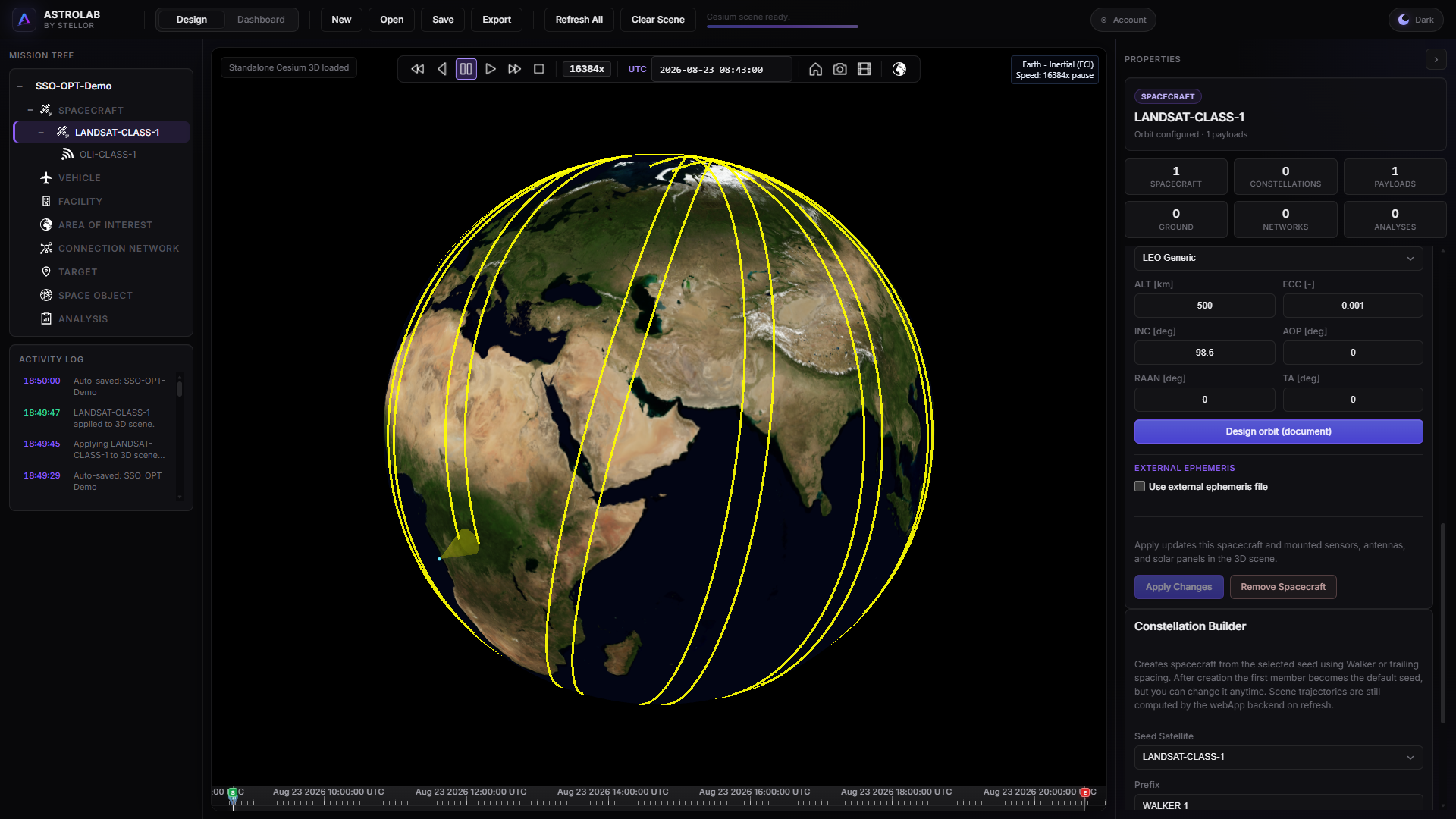
3D scene — spacecraft and optical sensor swath after Apply.
4 — Area of interest
- Right-click the Area of interest category → Add.
- Name it
AOI-USA. - In Countries, select United States of America.
- Apply Changes.
5 — Continuous coverage
Landsat-class missions acquire continuously along the sunlit ground track (land / coast), not as one-shot events. In ASTROLAB that is Coverage type Continuous.
Trial is for exploring the tool
The Trial exists so you can try ASTROLAB end-to-end — tree, orbit wizard, sensors, coverage, Dashboard — and see what the product can do. With a 12 h window and a 4° grid, results are intentionally coarse: they are not decision-grade coverage products. When you move to a higher plan you can lengthen the scenario, refine the mesh, and run analyses that actually deliver detailed engineering value.
- Right-click Coverage Analysis → Add. Name it
COV-SSO-1. - Type Continuous.
- AOI type = Area of Interest; select
AOI-USA. - Acquirers =
OLI-CLASS-1(the sensor, not only the bus). - Granularity 4°, computation Balanced.
- Run Analysis. Wait until it finishes.
If percent covered is still ~0, this 12 h phasing missed CONUS: widen the FOV a few degrees. A real Landsat swath needs 16 days to tile the continent.
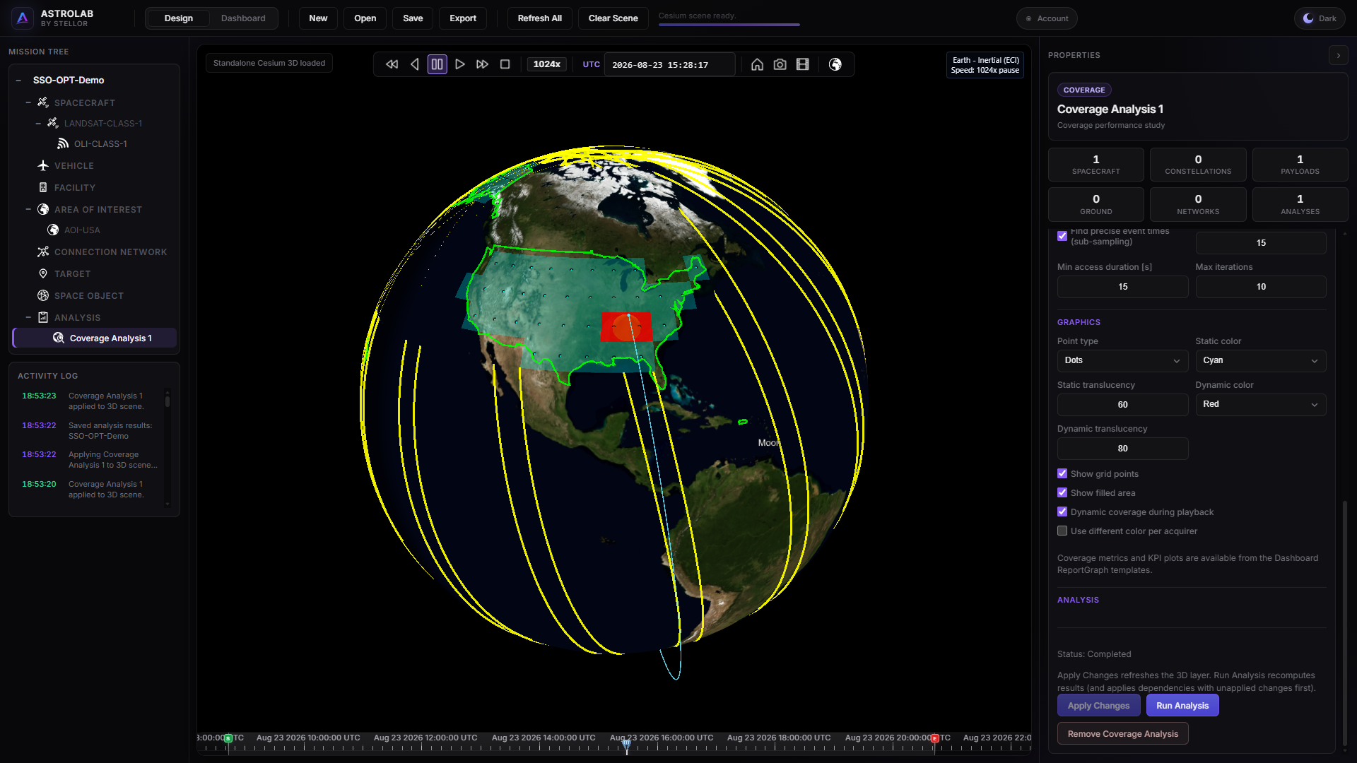
Continuous coverage — dynamic coverage overlay (red) over the USA AOI.
6 — Dashboard
- Top bar: Design → Dashboard.
- Asset =
COV-SSO-1(coverage templates live on the analysis, not only on the spacecraft). - Open Plots and pick a Continuous metric — for example Total Access as a heatmap.
- Click Generate Plot. You can also switch to Reports for tabular summaries.
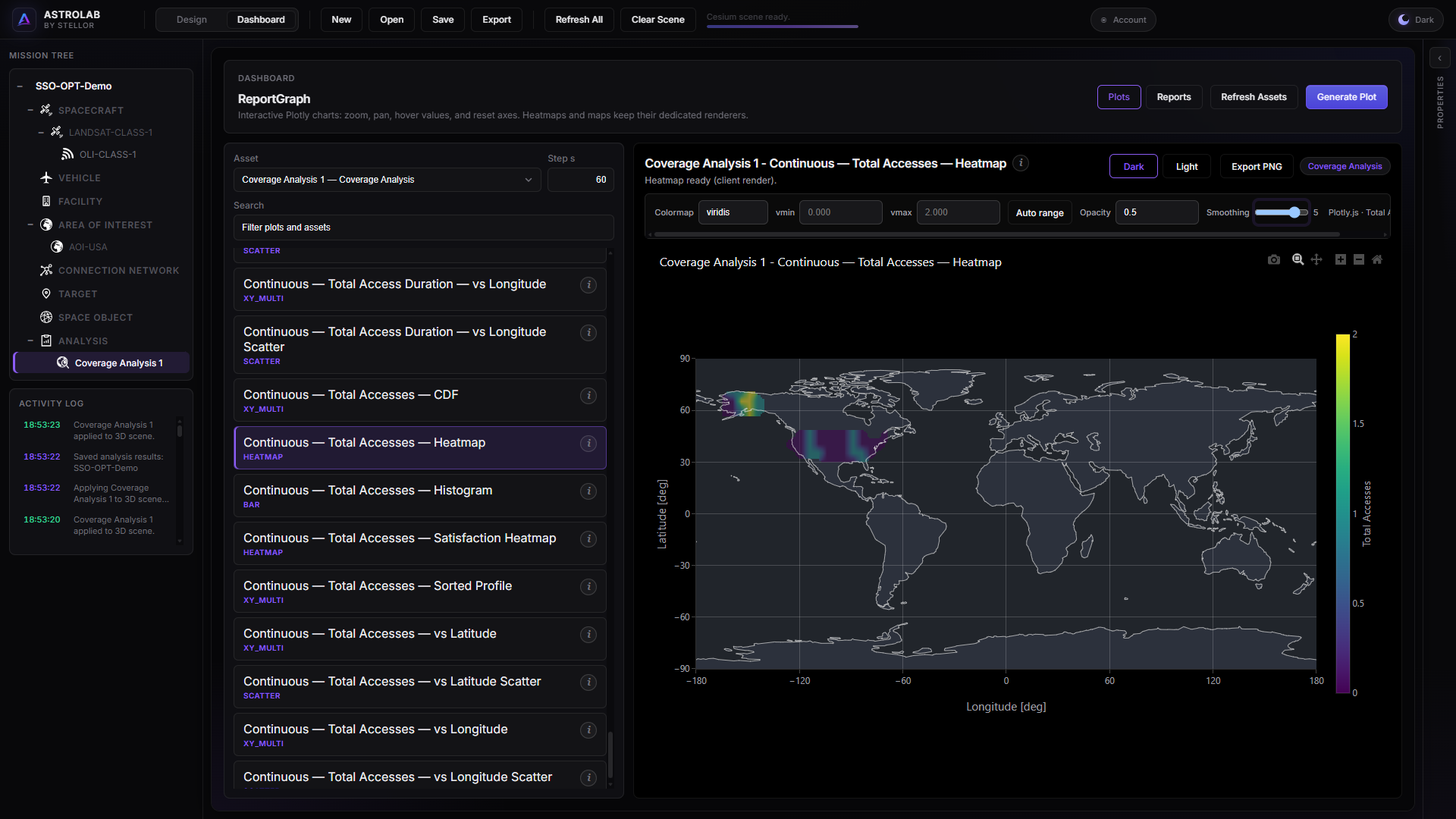
Dashboard — Total Access heatmap over the USA AOI.
Checkpoint
- SSO at ~705 km, morning MLTAN, nadir attitude.
- Optical sensor swath visible in 3D.
- Coverage Continuous completed with the sensor as acquirer.
- At least one Dashboard plot for
COV-SSO-1(e.g. Total Access heatmap).
Optional next (same mission)
| If you want… | Then… |
|---|---|
| Landsat-like swath | Half-angle ~7.5° and a longer scenario (beyond Trial 12 h) |
| Daylight-only collects | Constraint Target illuminated (or eclipse rules) on the sensor / coverage |
| Finer map | Granularity 2° + High Accuracy (plan permitting) |
| Lifetime of the bus | Separate Lifetime run with drag properties set |