Coverage
Regions and requests over the mission interval
Coverage answers how well your fleet serves a place or a set of requests. Link is one pair at a time. Coverage is the region, the grid, or the population of events.
Add it from the Mission Tree → Analysis → Coverage. Name it, choose type, pick who acquires, Apply Changes, Run Analysis.
Open Web App · walkthroughs: LEO Optical Satellite (Continuous) · LEO Radar Tasking (Discrete facility tasking)
When to use
| Use Coverage when… | Prefer something else when… |
|---|---|
| Percent of a country covered, gaps, heatmaps | One satellite–station pass → Link |
| IoT / imaging requests inside an AOI | Time to deliver after the look → Coverage then Latency |
| Radar-style command then look from a ground station | RF margin on one hop → Link with budget |
Three types
Pick Coverage type to match the operational question.
| Type | What it samples | Typical story |
|---|---|---|
| Continuous | A grid over the domain | Paint-the-Earth: revisit, percent covered, swath over a country |
| Discrete | Demand events (random or Poisson, in the AOI or born at a facility) | Messages, alerts, tasking — not every square kilometre equally |
| Static | A fixed set of points (count + seed) | Survey of N representative sites |
Finer Continuous grids and larger Discrete N cost more time and may be limited by your plan.
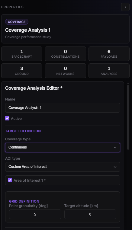
Coverage Properties — type, AOI, grid (Continuous).
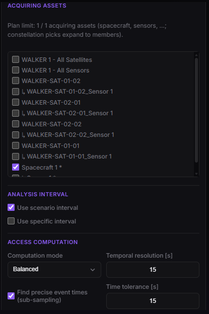
Coverage — Acquiring assets and computation method.
Who acquires
Check spacecraft, sensors, or constellation rows such as All Satellites / All Sensors. The engine expands a constellation to its members.
- Sensor — FOV and pointing matter (optical tutorial).
- Spacecraft only — geometric line-of-sight of the bus (radar-tasking tutorial: no sensor).
Inactive assets and constraints (elevation, eclipse, range) can zero the result without an obvious error.
Where on Earth
| AOI type (editor) | Meaning |
|---|---|
| Global | Whole Earth |
| Lat/Lon Region | Min/max latitude and longitude box |
| Custom Area of Interest | One or more AOI assets (countries, All Land, polygons) |
Computation (method)
Computation mode (Access computation) is how tightly the engine samples geometry over time. Other analyses that need access windows inherit the same idea — this page is the reference.
Picking a preset fills the fields below. Edit any of them and the mode becomes Custom.
| Mode | Typical use | What it actually sets |
|---|---|---|
| Fast | First look, long scenario, coarse grid | 60 s samples, no edge refinement. Short LEO contacts can be missed or discarded. |
| Balanced | Default for tutorials and most studies | 15 s samples and edge refinement. Good first-cut accuracy vs run time. |
| High Accuracy | Design decisions (plan-gated) | 10 s samples, tighter edges (1 s). Catches short passes; slower. |
| Custom | You own the numbers | Same fields, no preset. |
| Field (editor) | Meaning |
|---|---|
| Temporal resolution [s] | How often geometry is tested. Larger → faster, more likely to skip a short pass. |
| Find precise event times (sub-sampling) | Bisect between samples to pin contact start/end. Off in Fast. |
| Time tolerance [s] | How tightly that bisection may stop. Only with sub-sampling on. |
| Min access duration [s] | Contacts shorter than this are dropped. Fast uses 60 s — a 40 s LEO pass never counts. |
| Max iterations | Cap on bisection steps. Only with sub-sampling on. |
Graphics-only tweaks (colours, translucency) do not recompute. Changing compute settings invalidates a completed run (stale).
Continuous
A spatial grid over the AOI. At each time step the engine marks which cells are acquired, then accumulates statistics. Playback can show dynamic coverage on the globe.
| Field (editor) | Meaning |
|---|---|
| Point granularity [deg] | Spacing of grid cells. 4° is a Trial-friendly first look; finer grids resolve narrow gaps and cost more (plan may cap how fine). |
| Target altitude [km] | Height of the sample surface above the ellipsoid (0 = ground). Raise it only if you are covering an elevated layer, not the terrain. |
Use it for constellation comparison and sensor swath over a country. Coarse grids hide narrow gaps — tighten granularity before a design decision.
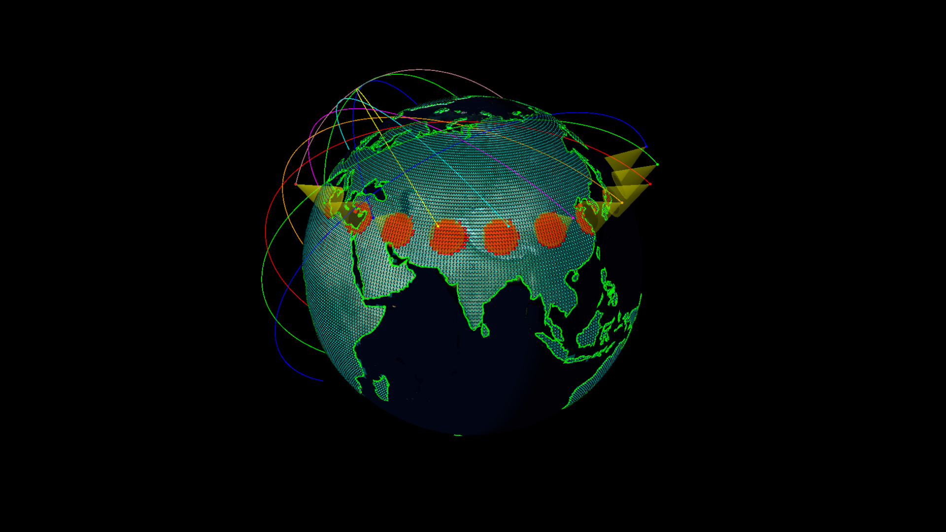
Design — Continuous coverage overlay on the AOI after Run.
Discrete
Events are drawn with a seed so the same N is reproducible.
| Field (editor) | Meaning |
|---|---|
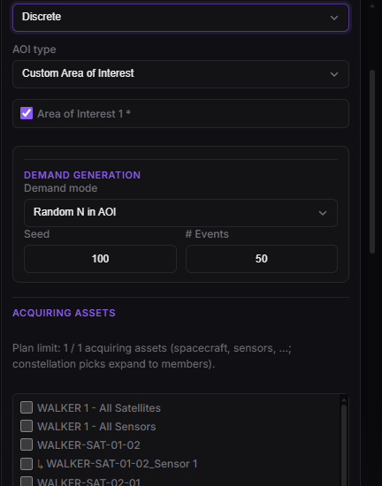
| Demand mode | Where requests are born (table below) |
| Seed | Random draw; same seed + same N → same points |
| # Events | Fixed population (non-Poisson modes). Plan may cap N. |
| Rate [Hz] | Poisson arrival rate instead of a fixed N |
| Demand mode | Where requests are born | What you measure |
|---|---|---|
| Random N in AOI | Inside the AOI | Time from birth to first see of that point (TOTAL) |
| Poisson in AOI | Stream inside the AOI | Same clock; rate instead of a fixed N |
| Facility tasking (N) | At checked tasking facilities | Same satellite must see the station first, then the AOI point |
| Facility tasking (Poisson) | Same chain, Poisson arrivals | Same two-leg story |
Facility-tasking points still lie in the AOI (the “look”); the facility is the command origin.
Delay clocks (facility tasking)
| Clock | Interval |
|---|---|
| TASKING | Birth → first see of the origin facility |
| ACQUISITION-LEG | That facility pass → first see of the AOI target (same satellite) |
| TOTAL | Birth → first see of the AOI target (the two legs added) |
AOI-born Discrete has no facility, so only TOTAL exists. Latency still picks up Discrete at TOTAL.
Delay CDFs only include successful contacts. Read chain outcomes (never tasked / tasked-no-image / acquired) for misses. A few Dashboard templates still say “Acquisition Delay by Acquirer” — they plot TOTAL, not ACQUISITION-LEG.
Design — Discrete events after a facility-tasking run.
Static
Static draws a frozen sample of sites inside the AOI and then treats those points like a sparse Continuous grid: they stay put for the whole interval. It is a survey of N places, not a live demand process.
That is the contrast with Discrete: Discrete events are born (random N or Poisson, optionally at a facility) and the clock is time-to-first-see. Static sites have no birth time and no facility-tasking chain — there is no TASKING / ACQUISITION-LEG / TOTAL table. Access, revisit, and gaps are accumulated over the scenario the same way as Continuous, but only at those N points instead of a regular degree grid.
| Field (editor) | Default | Meaning |
|---|---|---|
| # Targets | 500 |
How many sites to draw in the AOI. Plan may cap N. |
| Seed | 100 |
Random draw. Same seed + same N + same AOI → same sites. Change the seed to get another survey of the same region. |
AOI is the same Global / Lat/Lon Region / Custom Area of Interest as the other types — points are rejected until they land inside that domain.
| Use Static when… | Prefer Discrete when… | Prefer Continuous when… |
|---|---|---|
| You want revisit / access stats on a representative set of clients or towns | Requests arrive over time (IoT, alerts, tasking) | You need a field / heatmap over every cell |
| Latency Static traffic (fixed IoT packets or a continuous session) | Latency Discrete payload per event | Percent area covered, swath paint |
Latency linked to a Static Coverage uses these sites as the client locations (Fixed packet (IoT) or Continuous session).
On the globe, Static shows the sample points. Show filled area is Continuous-only (disabled here).
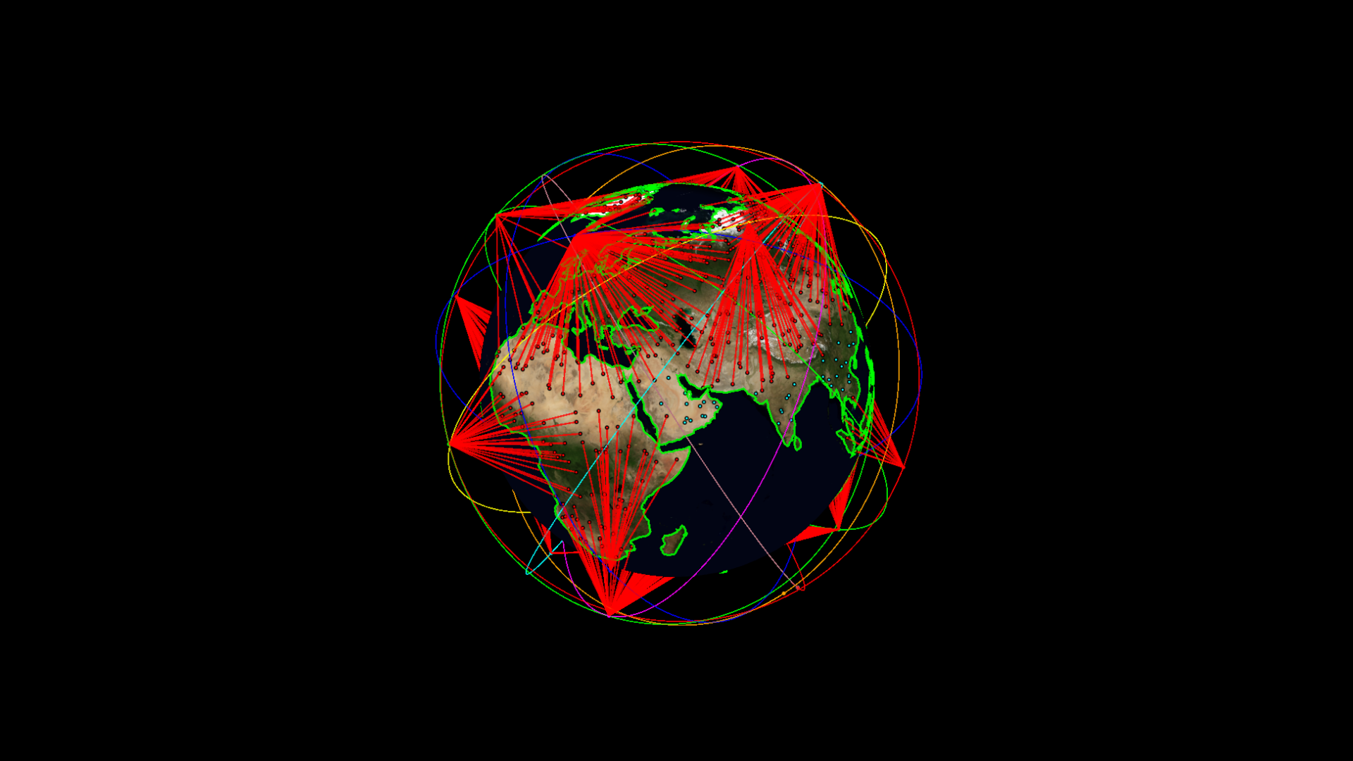
Design — frozen sample points after a Static run.
After Run
- Status completed.
- Design: grid, filled area, discrete events, or static sample points, depending on type.
- Dashboard: select this Coverage analysis — Continuous heatmaps; Discrete CDFs / chain outcomes; Static revisit at the sample sites.
Empty result: FOV, pointing, ground track vs AOI, constraints, who is checked as acquirer, or Min access duration longer than the pass — Troubleshooting.