LEO optical mission

Tutorial · TUT-EO-001 · Trial

The case

This exercise stands in for a small Earth-observation mission. One satellite flies a sun-synchronous orbit with MLTAN 0.5 h — 00:30 mean local time on the ascending node, so the ground track is on the night side. A nadir sensor with a 35° half-angle stands in for an infrared imager: a wide cone looking for temperature differences on the ground, for example land against water, or a warm patch against a cold background.

The bus writes what it sees into 100 MB files and dumps them to two polar stations, KSAT Svalbard and KSAT Troll. The rest of the page is how to build that mission in ASTROLAB. The globe below is the picture you should reach: the infrared swath on the Earth, and the two stations once they are in the tree.

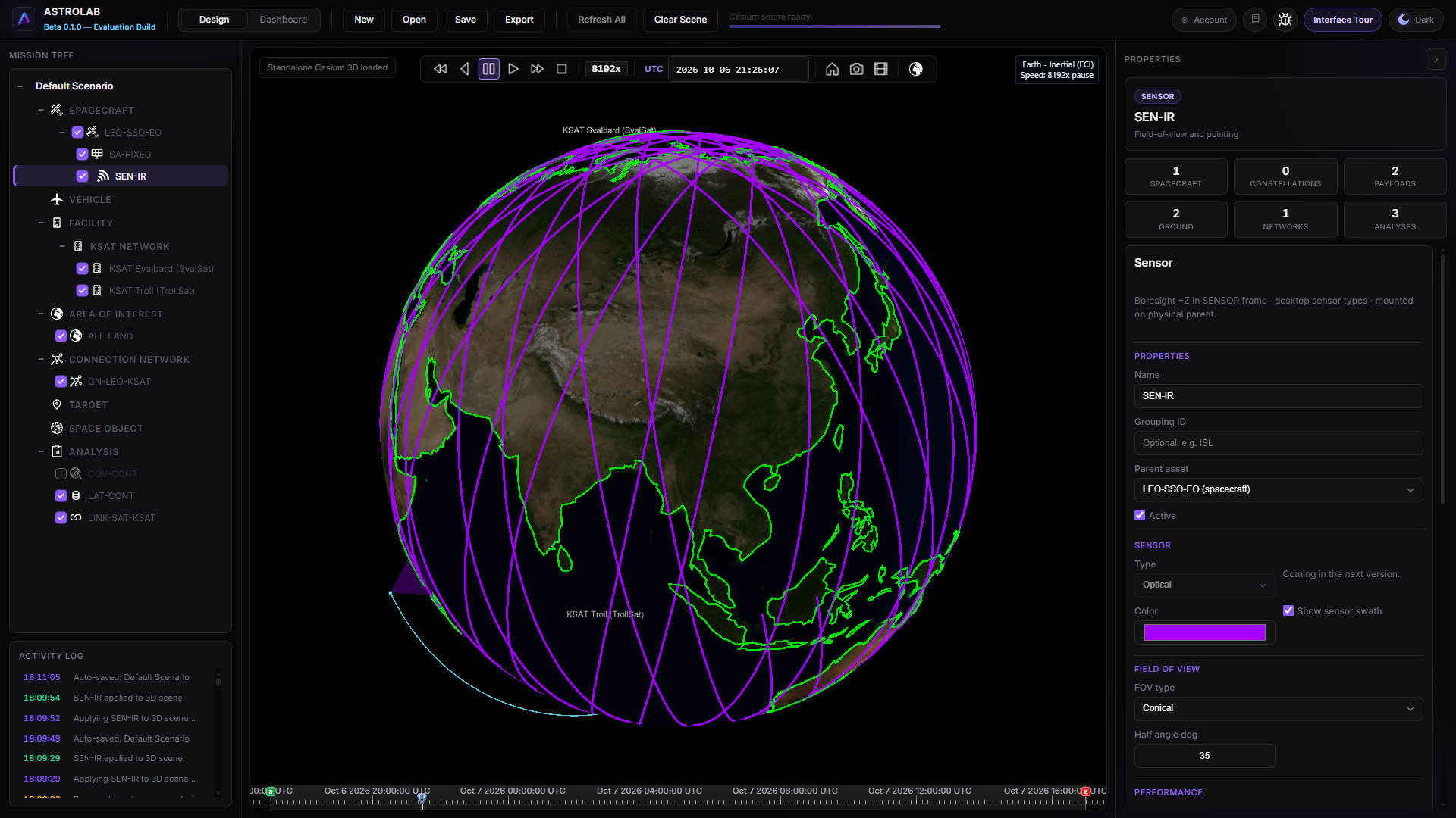
The case — SEN-IR swath on the night-side SSO, with KSAT Svalbard and KSAT Troll.

The finished mission is 24 h (6 Oct 2026 17:00 UTC → 7 Oct 2026 17:00 UTC), scenario step 120 s. That window fits the Web Trial. Do not go finer than 120 s on the scenario clock, and do not go finer than 3° on the coverage grid, or Trial will block the run.

Open Web App · start from Create your first mission

What you will build

1. Name the scenario TUT-EO-001 and keep the 24 h window.
2. Design spacecraft LEO-SSO-EO with the SSO repeating-ground-track wizard, attitude Nadir.
3. Add a body panel SA-FIXED and an optical sensor SEN-IR.
4. Add two KSAT stations and an All Land area.
5. Run a connection network, a continuous coverage, a link, and a latency study — in that order, because latency reads the other two.
6. Open the same plots in Dashboard.
7. Or skip the clicking and download the mission file.

What you type	Value
Scenario name	TUT-EO-001
Start / end	06/10/2026 17:00:00 UTC → 07/10/2026 17:00:00 UTC
Scenario time step	120 s
Spacecraft	LEO-SSO-EO
Orbit wizard	SSO Repeating Ground-Track — revolutions 59, cycle 4 days, MLTAN 0.5 h, TA 0
Attitude	Nadir
Panel	SA-FIXED, custom bus, mount face +Y
Sensor	SEN-IR, optical, conical half-angle 35°, acquisition rate 350 Mbps, body-fixed
Facilities	KSAT Svalbard (SvalSat), KSAT Troll (TrollSat)
Area of interest	ALL-LAND — global layer All Land
Connection network	CN-LEO-KSAT — LEO-SSO-EO → KSAT Network - All Stations
Coverage	COV-CONT, Continuous, grid 3°, acquirer SEN-IR
Link	LINK-SAT-KSAT — bus to both stations, link budget off
Latency	LAT-CONT — coverage COV-CONT, network CN-LEO-KSAT, closed file 100 MB

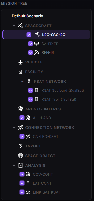
Mission tree when every step below is done.

1 — Scenario

1. New mission. Open Default Scenario.
2. Name it TUT-EO-001. The tree label updates as you type.
3. Set Start interval to 06/10/2026 17:00:00 UTC and End interval to 07/10/2026 17:00:00 UTC.
4. Set Scenario time step to 120. Central body stays Earth.
5. Apply Changes. Time bounds do not reach the globe until you apply.

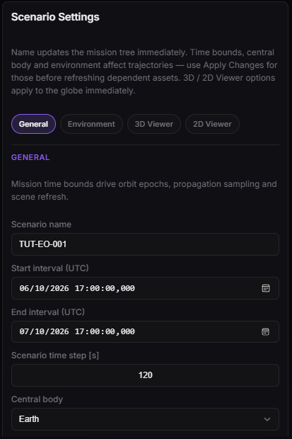
Scenario — name, 24 h window, step 120 s.

2 — Spacecraft and orbit

1. Right-click Spacecraft → Add Spacecraft. Name it LEO-SSO-EO.
2. Open the Orbit tab → Orbit design wizard.
3. Type SSO Repeating Ground-Track.
4. Revolutions 59, cycle 4 days, MLTAN 0.5 h, true anomaly 0.
5. Click Design orbit (document). The wizard writes the orbit into the state fields and shows a mean altitude (about 639 km). Check that the state changed before you leave the page.
6. Open Attitude → Nadir.
7. Apply Changes. The ground track should appear in 3D.

MLTAN 0.5 h is 00:30 mean local time of the ascending node. Leave it at 0.5 so your orbit matches this tutorial.

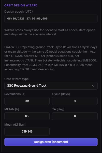
Orbit design wizard — 59 revolutions in 4 days, MLTAN 0.5 h, before Design orbit.

3 — Solar panel

The panel is part of the spacecraft body. You are not running a power study in this tutorial.

1. Stay on LEO-SSO-EO. Open Power.
2. Model source = Custom Design. Bus size 1 m × 1 m × 1 m.
3. Add panel. Asset ID SA-FIXED. Mount face +Y.
4. Apply Changes. SA-FIXED appears under the spacecraft in the tree.

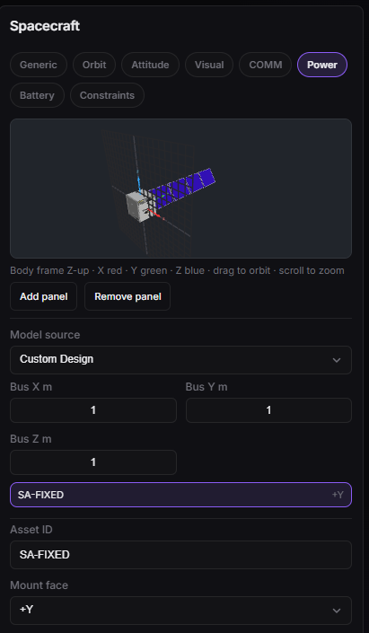
Power — custom bus and panel SA-FIXED on +Y.

4 — Optical sensor

1. Right-click LEO-SSO-EO → Add Sensor. Name it SEN-IR.
2. Type Optical. This is the infrared stand-in from the case: a wide cone, not a narrow visible camera. Turn on Show sensor swath.
3. FOV Conical, half-angle 35°.
4. Acquisition data rate 350 Mbps.
5. Mounting sequence 321, all rotations and offsets 0 (body-fixed, boresight along the bus).
6. Apply Changes.

In 3D the purple swath should match the globe at the top of this page. Switch the centre view to 2D for the map below.

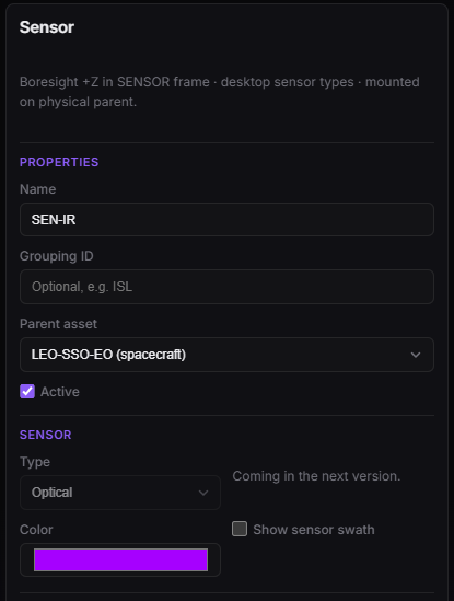
Sensor — name, optical type. Enable Show sensor swath before Apply.

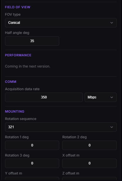
Sensor — conical 35° and 350 Mbps.

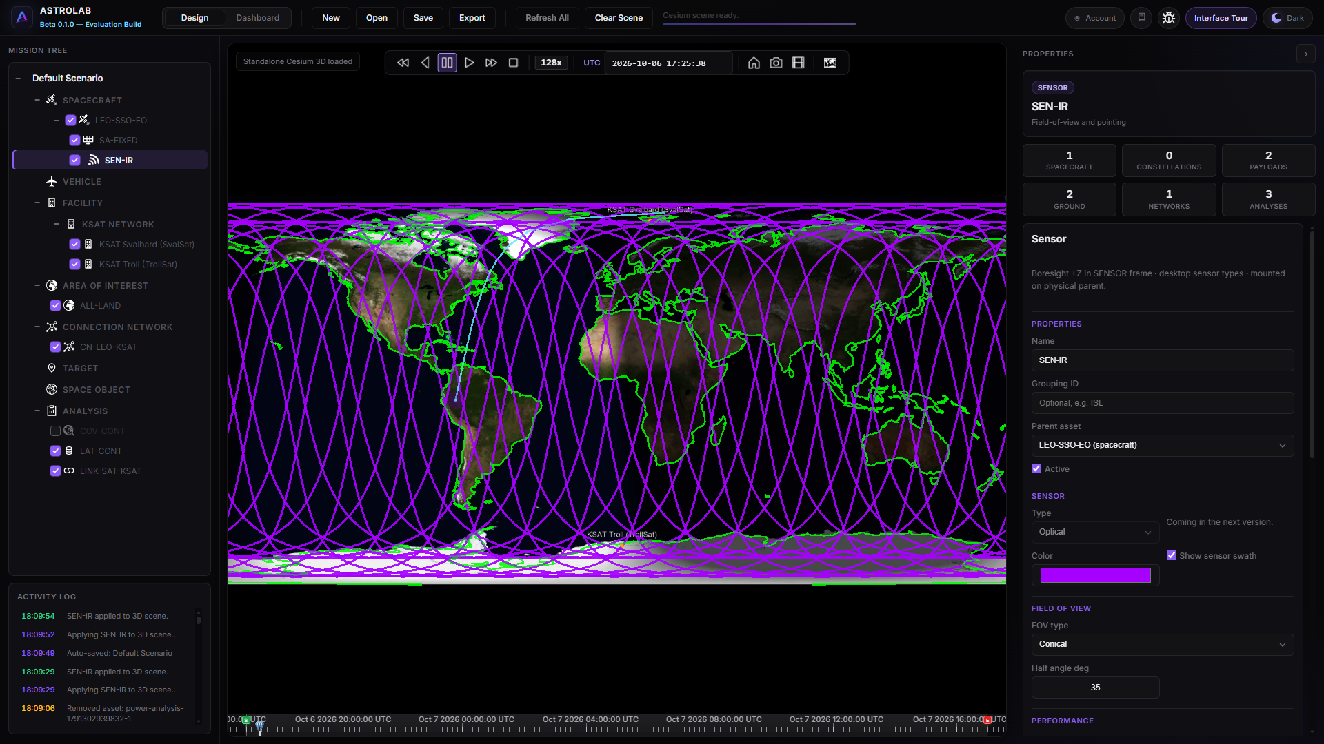
2D — same swath on the map.

5 — Two ground stations

Add each station as its own facility. Do not use Add entire KSAT Network — that would drop in every KSAT site. This mission only uses two, and they still group under KSAT Network in the tree.

1. Right-click Facility → Add.
2. Default database → KSAT Svalbard (SvalSat). Apply Changes.
3. Add a second facility. Default database → KSAT Troll (TrollSat). Apply Changes.

Leave the catalog elevation mask (5°). Both sites should sit under KSAT Network in the tree.

6 — All Land

1. Right-click Area of interest → Add. Name it ALL-LAND.
2. Under Global layers, check All Land only. Leave countries empty.
3. Apply Changes.

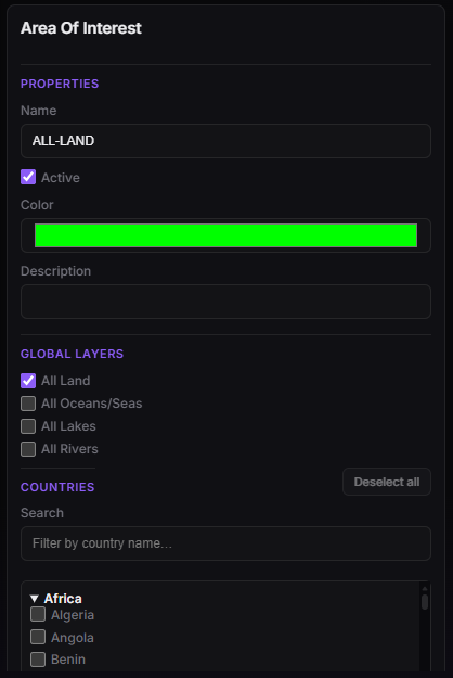
Area of interest — All Land, no country selected.

7 — Connection network

Latency needs this network. Build it before the latency study.

1. Right-click Connection Network → Add. Name it CN-LEO-KSAT.
2. Add one connection: From LEO-SSO-EO, To KSAT Network - All Stations.
3. Leave Use scenario interval on. Computation Balanced.
4. Apply Changes, then Run Analysis.

When it finishes, open Dashboard, asset CN-LEO-KSAT, and generate the access-window plot. You should see passes to Svalbard and to Troll.

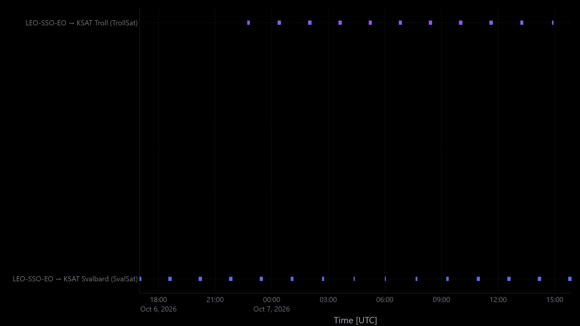
Dashboard — access windows for CN-LEO-KSAT.

8 — Continuous coverage

1. Right-click Analysis → add a Coverage analysis. Name it COV-CONT.
2. Coverage type Continuous. AOI type Custom Area of Interest. Check ALL-LAND.
3. Point granularity 3°. Target altitude 0.
4. Acquiring assets: check SEN-IR only (not the bus).
5. Use scenario interval. Computation Balanced, temporal resolution 10 s.
6. Apply Changes, then Run Analysis.

Back in Design, the coverage layer draws on the globe. In Dashboard, asset COV-CONT, generate the report and the two heatmaps below.

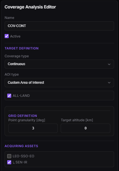
Coverage — Continuous, ALL-LAND, 3° grid, acquirer SEN-IR.

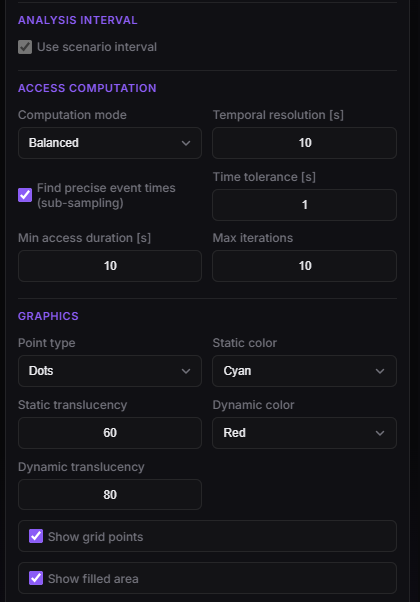
Coverage — scenario interval, Balanced, 10 s.

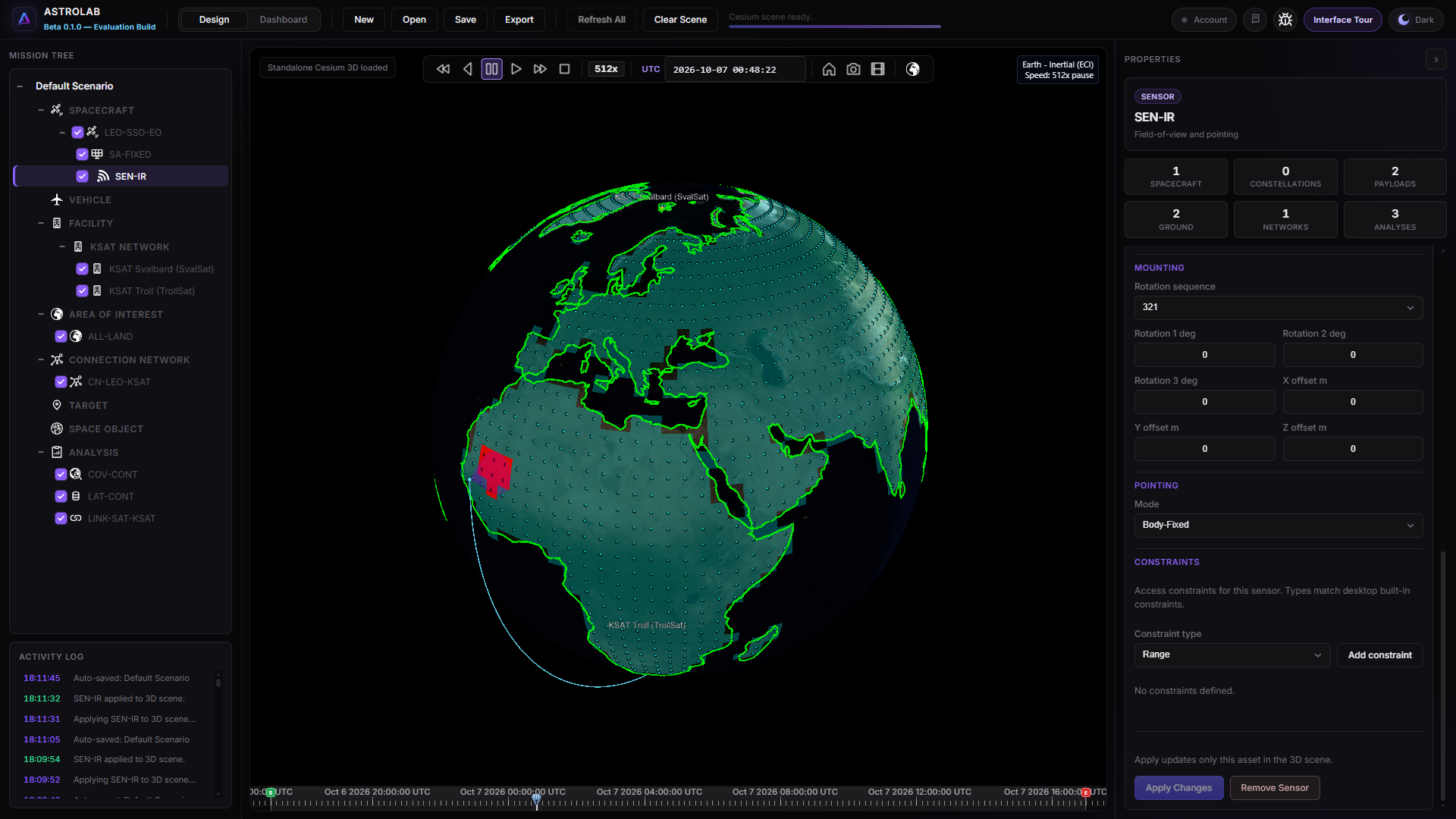
Design — COV-CONT drawn on the globe after the run.

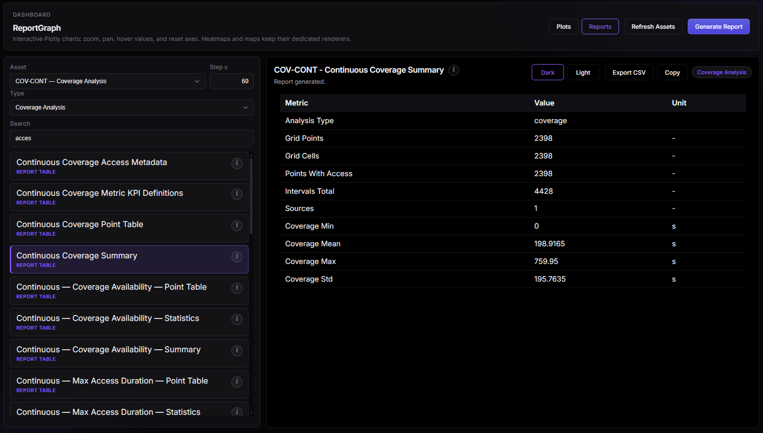
Dashboard — report for COV-CONT.

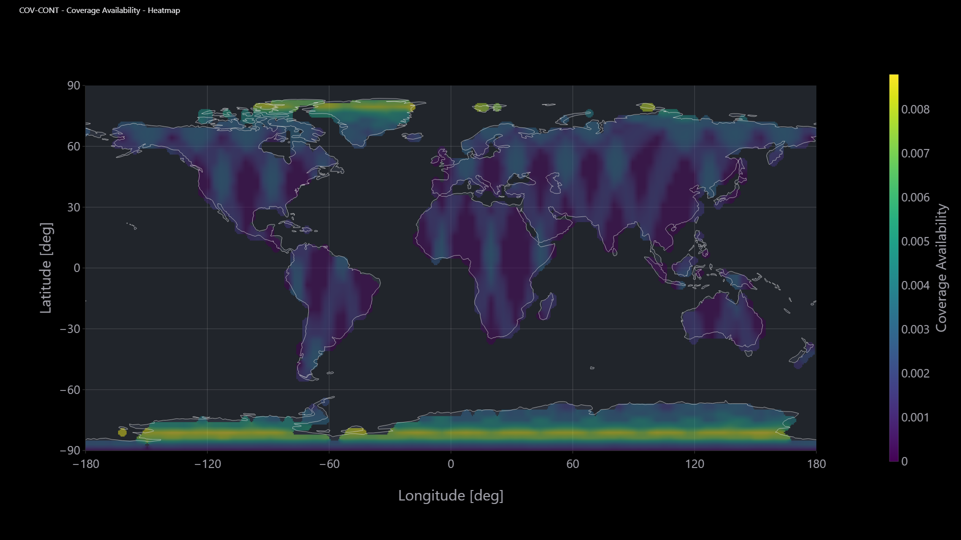
Dashboard — availability heatmap.

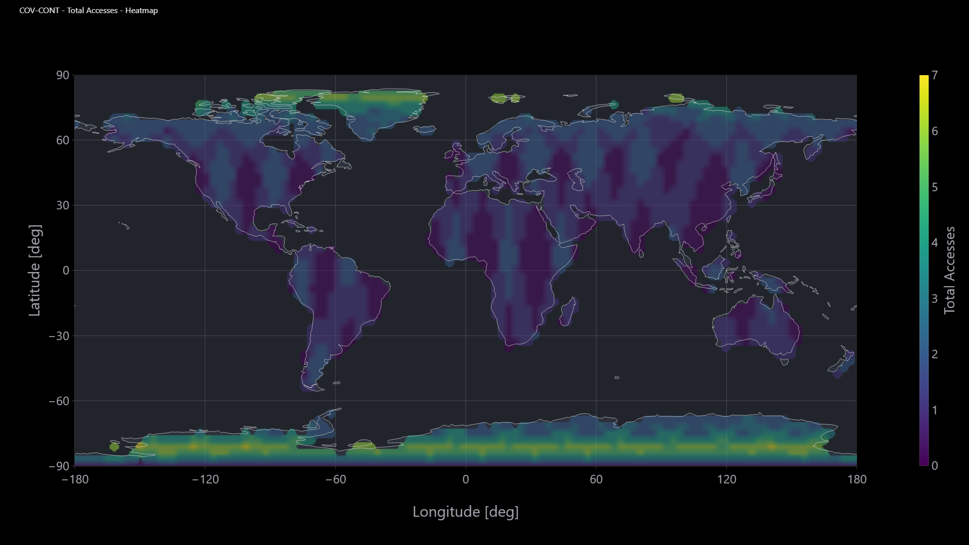
Dashboard — number of accesses heatmap.

9 — Link to the two stations

This study is the contact geometry between the bus and each station. Leave Compute link budget off — that box needs a transmitter, and this mission does not add one.

1. Add a Link analysis. Name it LINK-SAT-KSAT.
2. Primary asset: LEO-SSO-EO.
3. Secondary assets: KSAT Svalbard (SvalSat) and KSAT Troll (TrollSat).
4. Computation Balanced, temporal resolution 10 s.
5. Apply Changes, then Run Analysis.

In Dashboard, asset LINK-SAT-KSAT, generate the target sky plot.

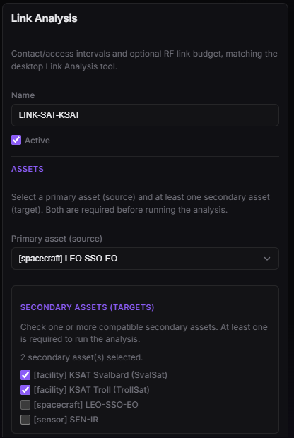
Link — bus to the two KSAT stations.

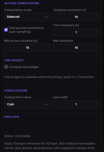
Link — Balanced access, link budget left off.

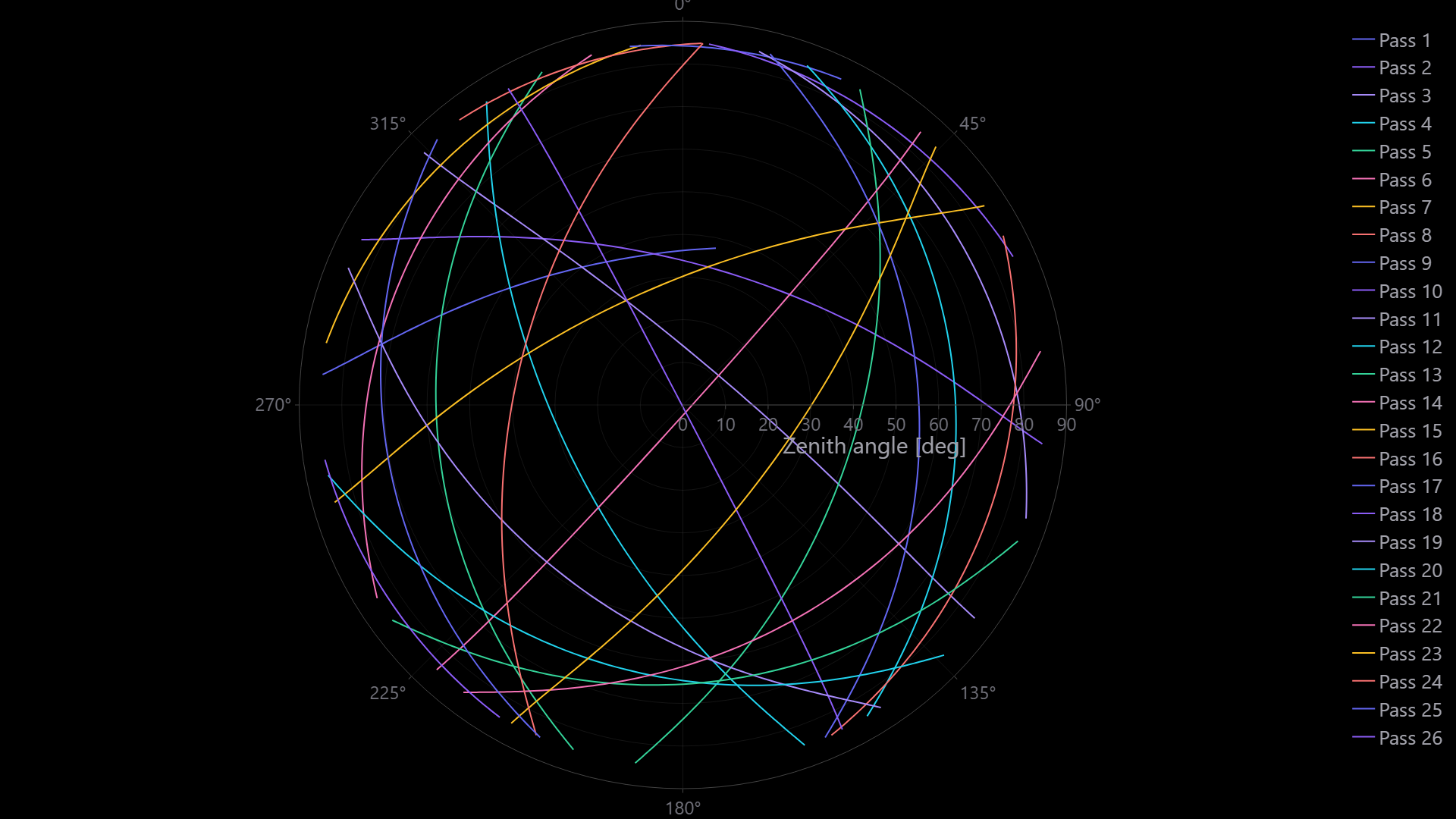
Dashboard — sky plot for LINK-SAT-KSAT.

10 — Latency

Run this last. It reads COV-CONT and CN-LEO-KSAT. If either study is still empty, latency has nothing to dump.

1. Add a Latency analysis. Name it LAT-CONT.
2. Coverage analysis COV-CONT. Connection network CN-LEO-KSAT.
3. Acquirers: Selected acquirers only → SEN-IR.
4. Ground stations: All facilities on network.
5. Dump routing: Direct downlink. Closed file size 100 MB.
6. Use scenario interval. Apply Changes, then Run Analysis.

In Dashboard, asset LAT-CONT, generate the delivery-delay CDF, the age-of-information plot, and the MMFU fill plot.

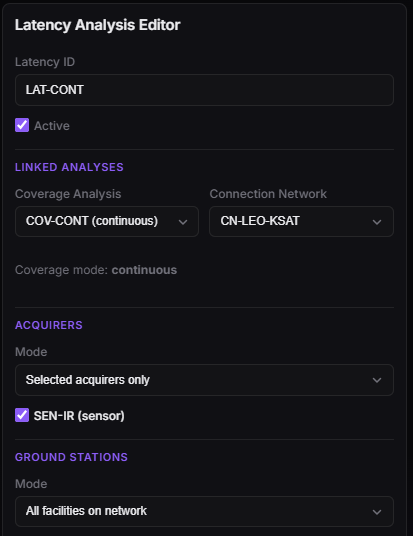
Latency — COV-CONT, CN-LEO-KSAT, acquirer SEN-IR.

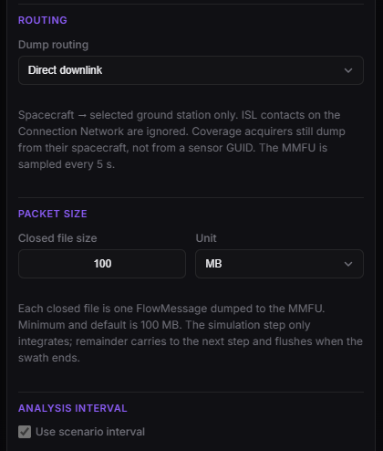
Latency — direct downlink, closed file 100 MB.

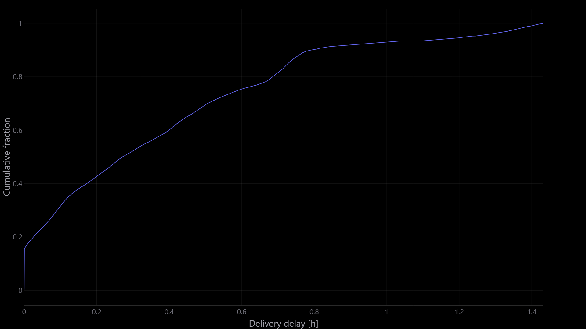
Dashboard — delivery-delay CDF for LAT-CONT.

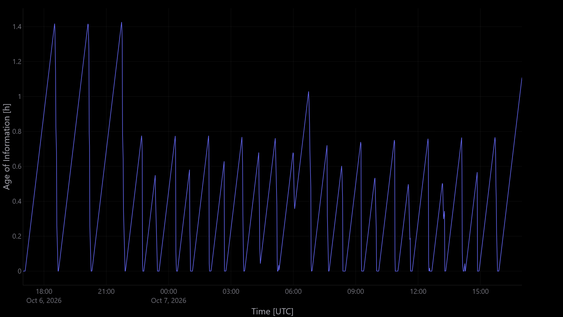
Dashboard — age of information.

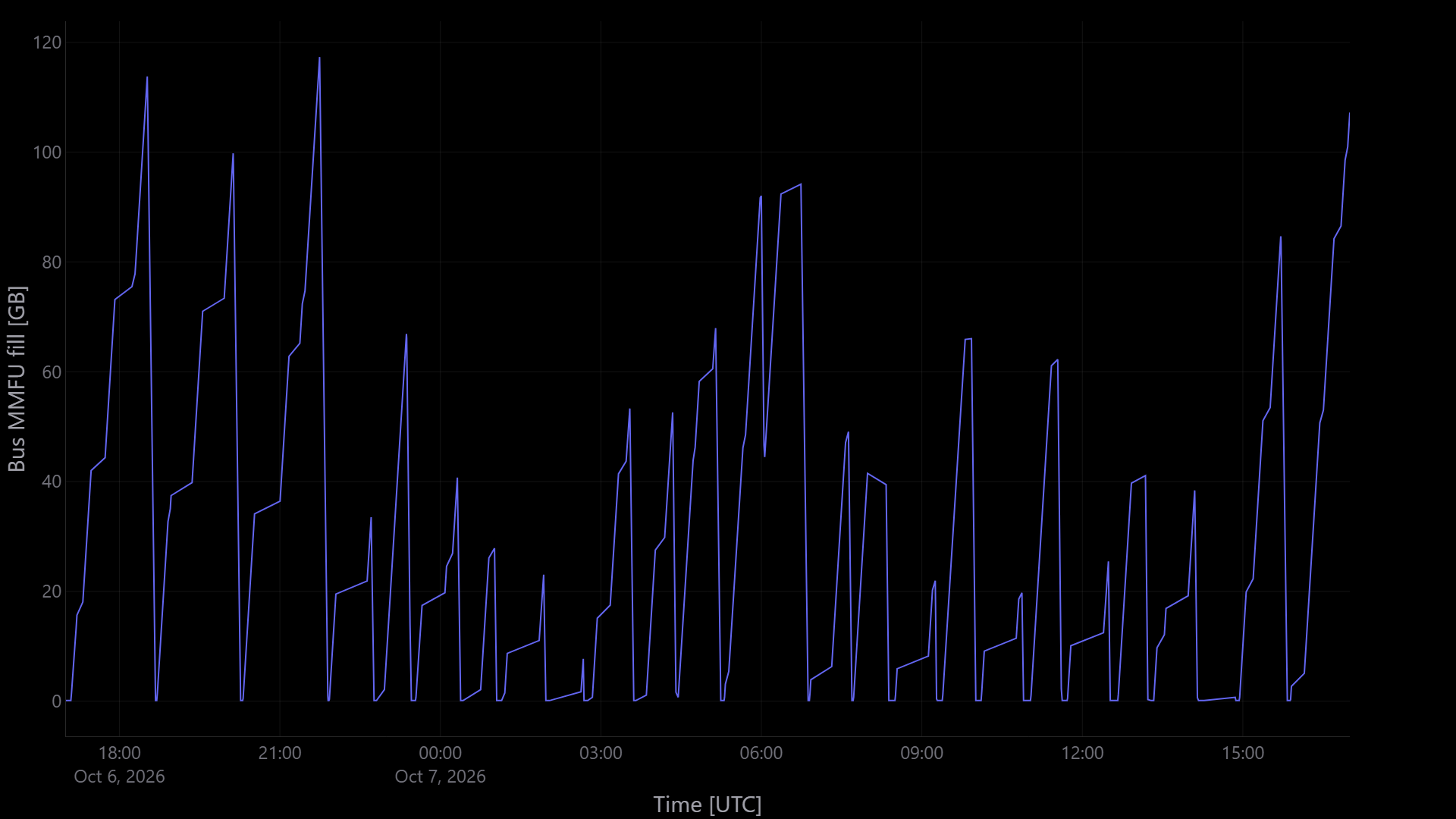
Dashboard — MMFU fill level.

Checkpoint

• Scenario TUT-EO-001, 24 h, step 120 s, applied.
• LEO-SSO-EO on the designed SSO, nadir, with SA-FIXED and SEN-IR.
• Two KSAT stations under KSAT Network, and ALL-LAND.
• CN-LEO-KSAT, COV-CONT, LINK-SAT-KSAT, and LAT-CONT have been run.
• Dashboard shows the access windows, the two coverage heatmaps, the sky plot, and the three latency plots.

Download the mission

The same mission, already run, is in this folder. Top bar Open, then choose the file. You land on the tree in the figure above and can change any step and run it again.

Download TUT-EO-001.astrolab

Related

• Spacecraft · Sensors · Solar array · Facility · Area of interest
• Connection network · Coverage · Link · Latency · Reporting

Version

Written and checked on ASTROLAB Beta 0.1.0, on the Trial plan. The steps, the figures, and TUT-EO-001.astrolab match that build and those limits (24 h, step 120 s, coverage grid 3°). See the Beta 0.1.0 release notes and Plans and entitlements.